Author's Note

This blog post is part one in a series originally put together for the University of Victoria's CSC 460 course. The original content was published February 6 2019 by Torrey Randolph and myself. As that webpage no longer exists I am now hosting the content here.

Here are links to part 2 and part 3.

The goal of project 1 was to familiarize ourselves with the hardware and software interfaces we would be using throughout the semester. This project was broken in to two phases, details of which are provided below. This introductory section breaks down the software, hardware, and shared design decisions that were used to complete project 1.

In phase 1 we integrate these elements into a working solution. We control and aim a laser using an analog stick and detect the laser using a photocell. In phase 2 we create a similar solution, only this time we split the components across two boards and connect them together over Bluetooth.

We took advantage of the software ecosystem provided by companies like Atmel and Arduino, as well as community created tools and libraries. Here are the major dependencies we used.

• VS Code: We opted to move away from Arduino IDE to a more developed code editor after completing exercises 1 through 5. Visual Studio Code offered a development experience our team was familiar with as well as helpful extensions for working with Arduino hardware.
• AVR Toolchain: In order to compile code to our board outside Arduino IDE we make use of avr-gcc, a version of the GNU Compiler Collection specifically built for AVR micro-controllers. AVR Libc is the backbone of the Arduino libraries. We included the source code of relevant Arduino libraries with our projects for ease of integration with hardware. These libraries include ArduinoCore-avr, Servo, and LiquidCrystal. The defacto method of uploading and downloading software to AVR boards is AVRDUDE. We use the Arduino IDE configuration file for convenience and ease of use.
• Mekpie: Our project is built using Mekpie. Mekpie is a simple C build tool written by one of our members that was updated to support building software for AVR boards.
• Saleae Logic: This is the software tool used for recording values via a Saleae USB logic analyzer. This tool is essential to collecting real-time data with little to no overhead.

Our project made use of the following pieces of hardware. We combined this hardware using the usual suspects, breadboards, wires, and resistors.

• 2x Arduino Mega 2560 boards: Only one of these was needed in phase 1, but phase 2 required the creation of a base and remote station.
• 2x SG-90 Micro Servos in a pan and tilt module: These two servos are used to aim a mounted KY-008 Laser.
• 2x HC-06 Bluetooth modules: These two Bluetooth modules are used to communicate between the base and remote stations in phase 2.
• Arduino LCD KeyPad Shield: The Liquid Crystal Display is used to display relevant information, such as the current X and Y values of the analog stick.
• Arduino KY-023 Joystick: An analog joystick used to control the motion of the pan and tilt module.
• KY-008 Laser: This laser is used to shoot at our photocell.
• photocell: Used to detect the laser.

The AVR processor does not have built in support for floating point types. As a consequence, floating point operations are achieved using software. This has the drawback that performing floating point arithmetic is significantly slower than integer arithmetic, transforming 1-cycle instructions into 200 plus cycle instructions. This had a noticeable performance impact during exercise 4 when contrasting floating point analysis of an analog signal to integer analysis. When considering performance and our overarching goal of achieving low power consumption, it is in our interest to have as few floating point operations in our solution as possible.

When considering how to approach calculations typically done with floating point types, such as a low pass filter, we decided that fixed point operation may fit our needs.

Fixed point types can be considered integer values that are scaled up and down to represent smaller values. For instance, a fixed point scale of 10 would mean that 15 represents 1.5, and 57 represents 5.7. For efficient transformation to and from a fixed point format embedded programmers typically use a scale that is a power of 2. This allows scaling to be done by bit shifting. Fixed point numbers used in this way are typically expressed in the form QI.F where Q is the "sign" bit (in the 2's complement sense), I is the integer bits, and F is the fractional bits. So our chosen fixed point format of Q7.8 translates to a 16-bit value of the form:

The implementation of the data type is quite straightforward. Q7.8 corresponds to a scale of 0x0100.

// [-128.996, 127.996]
#define Q78_SCALE_FACTOR 0x0100

// Q7.8
typedef s16 Q78_t;

#define Q78(n) ((Q78_t) ((n) * Q78_SCALE_FACTOR))

We provide a type definition and a conversion macro for convenience. A macro is used rather than a function to allow for optimization of numeric constants. If a fixed point number is immediately added to or subtracted from a numeric constant and it is initialized using a macro, the numeric constants can be pre-applied by the compiler.

Fixed point numbers have several advantages, the first being that addition and subtraction are trivial. Integer addition and subtraction of fixed point values sharing the same scale work without additional effort. Multiplication and division requires a little more work, but not much.

Q78_t Q78_mul(Q78_t a, Q78_t b) {
    s32 tmp_a = a;
    s32 tmp_b = b;
    s32 tmp_c = (tmp_a * tmp_b) / Q78_SCALE_FACTOR;
    return (Q78_t) tmp_c;
}

Q78_t Q78_div(Q78_t a, Q78_t b) {
    s32 tmp_a = a;
    s32 tmp_b = b;
    s32 tmp_c = (tmp_a * Q78_SCALE_FACTOR) / tmp_b;
    return (Q78_t) tmp_c;
}

Q78_t Q78_lpf(Q78_t sample, Q78_t average, Q78_t factor) {
    static Q78_t one = Q78(1);
    return Q78_mul(sample, factor) + Q78_mul(average, (one - factor));
}

The key to these operations is ensuring that you do not overflow your intermediate values, hence both multiplication and division use 32-bit integers for intermediate values. In addition to multiplication and division operations, we also implement a simple low pass filter using fixed point values.

The core drawback of fixed point numbers is their limited range. For Q7.8 we can represent values between -128.996 and 127.996. This means that wherever we take advantage of fixed point numbers in our project we must ensure that our operands and results fit within that range.

The implementation of fixed point discussed here is based off a series of online lectures on the topic by Eli Hughes. Fixed point numbers are just one solution in a sea of possible ways of representing and computing the results of fractional arithmetic. We also looked into rational number formats, but ultimately preferred fixed point representations because of their simplicity.

The goal of phase 1 was to use an analog stick to control and aim a laser to shoot a photocell that could subsequently detect the shot. All of these components were integrated using a single Arduino board. Thanks to the five exercises completed prior to phase 1. producing our solution was a smooth process. The block diagram below shows the general setup of our system.

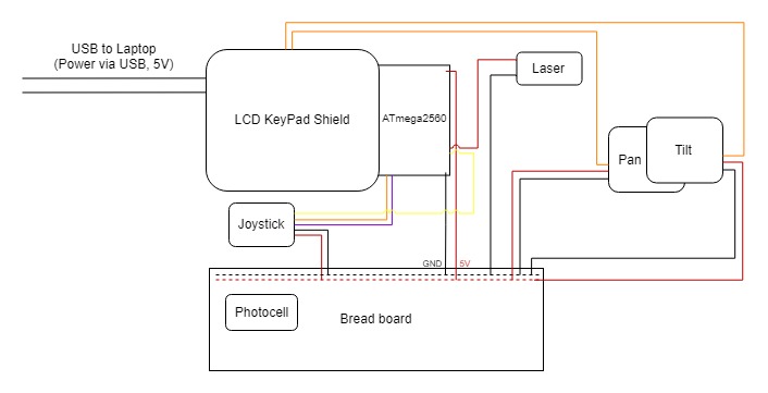
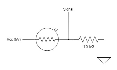
A 10kΩ resistor was used to create a voltage divider for our photocell. As the resistance of the photocell changes when light is shone on it, the voltage across the 10kΩ resistor changes. That voltage is reported by the Mega 2560, mapped to the range (0, 1023). When the photocell is hit by the laser, the voltage reported increases to above a certain threshold, which was determined by trial and error.

Phase 1 featured a simple main loop where we sample the analog stick, adjust the servos, toggle the laser, and then check if our photocell has been hit. There are no delays in this process so we simply try to go through these steps as quickly as possible, and then repeat. This is a poor solution when considering power consumption, as the CPU is never idle. It is important that the LCD is only updated when the photocell actually changes state. We discovered this in an earlier implementation where updating the LCD on every iteration of our main loop resulted in an unintelligible output from the LCD.

for (;;) {
    map_servo_pan(sample_stick_u_x(), 0, STICK_U_OFFSET_X);
    map_servo_tilt(-sample_stick_u_y(), 0, STICK_U_OFFSET_Y);
    if (stick_u_down()) {
        set_laser(ON);
    } else {
        set_laser(OFF);
    }
    if (photocell_hit()) {
        lcd.clear();
        lcd.print("Hit :O");
        set_laser(OFF);
        break;
    }
}

Our sampling method for the analog sticks was established during exercise 4. We use a combination of a low pass filter and a clamp. For efficient computing, these computations are performed using fixed point values. After reading the raw analog value, we scale it down so that it will fit within the fixed point range, and then offset it so that the values are centred at 0. This makes more efficient use of the signed fixed point range.

After reading, scaling, and offsetting our value we pass it through a simple low pass filter. The low pass filter is implemented as a simple rolling average function. Passing the value through the low pass filter reduces noise and gets us smoother feeling control with the stick. We pass all values into the low pass filter, including those that fall into the dead zone. This increases the accuracy of our rolling average.

The previously mentioned dead zone is a small region around the zero signal of the stick, that is clamped down to 0. This clamping combats two issues with analog inputs. The first is that the sticks have some noise in their input signal, even when at rest. This means that the measured value can be greater or less than 0 even if no one is touching the stick. Additionally, the sticks do not always come to rest at the exact same position due to friction, wear, and manufacturing imperfections. A dead zone mitigates these issues.

Our dead zone is implemented using a clamp. We similarly clamp the maximum value slightly below the theoretical maximum. This ensures that when you push the stick to the furthest edge in any direction we return the same maximum value.

Putting all of these decisions together we end up with the following implementation.

int sample_stick_u_x() {
    static Q78_t rolling_x = Q78(0);
    static Q78_t sample_x  = Q78(0);
    sample_x  = Q78((analogRead(STICK_U_PIN_X) - STICK_U_OFFSET_X) / STICK_SCALE);
    rolling_x = Q78_lpf(sample_x, rolling_x, STICK_LFP_FACTOR);
    int x     = Q78_to_int(rolling_x);
    if (x < 0) {
        x = clamp(x + STICK_U_DEADZONE, STICK_U_MIN_X, 0);
    } else if (x > 0) {
        x = clamp(x - STICK_U_DEADZONE, 0, STICK_U_MAX_X);
    }
    return x;
}

Correctly performing these operations requires we measure out constants for each analog stick. Namely their minimum, maximum, and resting values. We determined these values using a separate program, and recorded the constants for each of our two sticks. This ensures we are obtaining the highest quality samples possible.

We map the stick values to the servo positions in an intelligent manner. The servo is moved in discrete steps. These steps enforce a maximum delta in position and a minimum delay between changes. This protects the servo from having its position changed too rapidly, which could damage it.

The implementation first checks to see if the servos are ready to have their positions changed again; this is done by keeping track of the last time they were called using Arduino's millis function. If sufficient time has passed we change the input into a fractional value between 0 and 1 and multiply this by our maximum delta. This means that small changes will map to slow rotation of the servo and large changes will map to fast rotation of the servo. We also clamp the delta again to ensure that we do not exceed our maximum delta due to incorrect arguments. Finally, we clamp the position before writing it to ensure we do not move the servo past its maximum range. Most of these operations are performed with fixed point values for efficiency.

void map_servo_pan(int value, int min_value, int max_value) {
    static int servo_pan_position = SERVO_PAN_CENTER;
    static int last_call = 0;
    int this_call = millis();
    if (this_call - last_call < SERVO_PAN_DELAY) {
        return;
    }
    last_call = this_call;
    Q78_t range = Q78(SERVO_PAN_MAX_SPEED);
    Q78_t ratio = Q78_div(Q78(value - min_value), Q78(max_value));
    Q78_t delta = Q78_mul(range, ratio);
    servo_pan_position += clamp(Q78_to_int(delta), -SERVO_PAN_MAX_SPEED, SERVO_PAN_MAX_SPEED);
    servo_pan_position =  clamp(servo_pan_position, SERVO_PAN_BOTTOM, SERVO_PAN_TOP);
    servo_pan.writeMicroseconds(servo_pan_position);
}

The goal of phase 2 was to separate the components into two stations, each with a Mega 2560 board and have them communicate over Bluetooth. Below are block diagrams of the two stations.

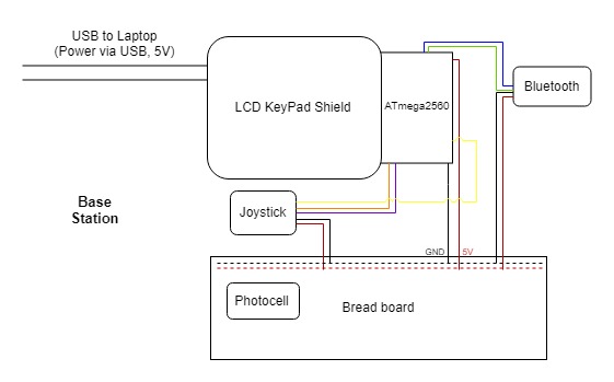
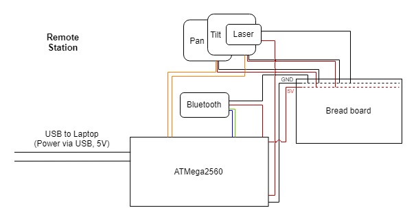
The base station includes the LCD, the joystick, the photocell, and one of the Bluetooth modules connected to a Mega 2560. The remote station consists of the pan and tilt servo motors, the laser, and the other Bluetooth module connected to another Mega 2560. The base station sends the joystick position to the remote station, which updates the servo motors and the laser positions correspondingly. In our implementation, the base station also sends a done flag when the photocell is hit by the laser to indicate that the program should gracefully shut down.

Phase 2 is to be implemented using a time triggered architecture (TTA). We make use of a scheduler developed by Neil MacMillan, a former TA of this course. In a TTA, tasks, implemented here as C functions, are run on a set period. In between these tasks the CPU is simply left to idle. A TTA has a number of benefits to real-time systems.

• They are deterministic; a correct schedule will remain correct ad infinitum.
• They are simple, especially compared to preemptive schedulers.
• They are lightweight, as the scheduler itself has very little bookkeeping to accomplish.

The choice of a TTA led us to the decision of avoiding interrupts in both phase 1 and 2. TTA nicely integrates with polling-based algorithms, so for all our inputs and communication we use polling rather than interrupts to keep up with IO.

In our implementation the base station and remote station both alternated between two tasks. The base station had the task sample for collecting input from the analog stick and photocell, and send for packaging that information together and sending it over Bluetooth. The remote station had the task receive for collecting the information sent from the base station and control for using that information in the activation of the laser and servo motors. The actual implementation of these tasks rely on the same code presented in phase 1.

We elected to sample our analog stick at approximately 60Hz. This was done based off the knowledge that responsive video games typically target 60 frames per second. We then match this rate in sending out the input information to the remote station. In retrospect, it would be worth investigating sampling at an even higher rate, and sending at the same or slightly slower rate. The logic being that the low pass filter we apply to our analog stick input would be most effective on an over sampled input.

On the remote station we faced a number of issues actually receiving a message. We hypothesized that this was due to two core problems:

1. The Bluetooth and/or UART pin on the board had a limited buffer which could overflow and produce unexpected results.
2. The first byte sent by our base station did not always correspond to the first byte read by our remote station.

Part of the reason these two problems caused us so much pain was that we had elected to communicate by sending a struct over Bluetooth. This meant that getting the correct values depended completely on byte order, unlike in something like a JSON encoding, where the relative position of data could be preserved.

When developing our solution, the first of these problems caused a number of strange behaviours, such as a massive delay between the initial push of the analog joystick and the servo activating, as well as the remote station randomly indicating it had been sent the done signal. These issues went away once we over sampled our Bluetooth signal (we landed at a rate of about 100Hz). This prevented the Bluetooth buffer from growing too large which caused delay, and upon overflow, incorrect values. Because we prevent our receive task from reading the next message until the servos have been given new values, we also had to have our control task update at a similarly high rate. In the future it may be worth exploring a slower control rate combined with aggregating received messages.

The second issue of byte alignment we solved by developing a simple communication protocol.

A struct was used to communicate our data over Bluetooth. We used a four byte header for alignment. Shown below are the definitions of the struct and relevant constants.

#define MESSAGE_HEADER ((u32) 0x04030201)
#define MESSAGE_DONE   0b00000001
#define MESSAGE_LASER  0b00000010

typedef struct Message Message;
struct Message {
#ifdef MESSAGE_SENDER
    u32 header;
#endif
    s8 u_x;
    s8 u_y;
    s8 m_x;
    s8 m_y;
    u8 flags;
};

For our data values we selected as efficient of integer types as reasonably possible. Our analog stick values come from fixed point calculations, meaning they are guaranteed to be between -128 and 127, which means a single signed byte is all that is needed to communicate each stick position. We send the done flag and laser state in a single shared byte, as this is the smallest reasonable encoding for that binary data.

The 4-byte header provides a means of synchronizing the remote and base stations. Having the remote station wait until it has correctly read the header will help guarantee data correctness. We started with an 8-byte header that simply counted from 1 to 8. Immediately we ran into an issue of endianness, as a u64 of 0x0102030405060708 is actually encoded low byte first in memory on our boards. Since we were reading these bytes one at a time at the remote station we had to reverse the order of our header value. Once we had a working system we lowered the header down to 4 bytes and found there was no loss in correctness. More clever schemes for alignment could be devised. Two that we considered are as follows:

• The Bluetooth modules seems to provide a reliable connection, meaning we could attempt to synchronize only once at startup and then trust that we will receive every byte in alignment.
• We could use a single byte for alignment, such as 0xFF, and to ensure correctness enforce the policy that all fields of our message struct are never allowed to encode this value.

Ultimately, we preferred our solution for its simplicity and reliability. In terms of implementing this protocol, the main work rested on the remote station. Its process of receiving bytes can be modeled using a simple state machine, shown below.

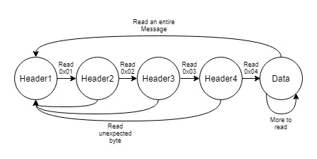
The four-byte header precedes each message. One drawback to this design is that if the remote station misses the header for any reason, that message will be skipped and the information will be lost. If the remote station successfully sees the header, the next five bytes it reads will be the message data, which it will subsequently map to servo positions and the laser state.

The implementation of send for this protocol is provided below. We send the struct byte by byte over Bluetooth. If we assume our receiver will similarly copy our bytes into a buffer of the same type, this has the nice feature of not caring about endianness, so long as the client and host agree.

void send() {
    digitalWrite(LOGIC_SEND, HIGH);
    // Write each byte of current message onse at a time
    u8 * buffer = (u8 *) &current_message;
    u16 i;
    for (i = 0; i < sizeof(Message); i++) {
        Serial1.write(buffer[i]);
    }
    digitalWrite(LOGIC_SEND, LOW);
}

The receive function is slightly more complex. First it must correctly implement the aforementioned state machine, as well as the function should not block if serial input from the Bluetooth is not available. The later issue is nicely resolved using static variables. For ease of implementation we generalize the first four states into a single handler.

void receive() {

    static int i = 0;
    static int state = header1;

    digitalWrite(LOGIC_RECEIVE, HIGH);
    if (current_message == NULL) {
        u8 * buffer = (u8 *) &buffer_message;
        while (Serial1.available()) {
            switch(state) {
                case header1:
                case header2:
                case header3:
                case header4:
                    if (Serial1.read() == state) {
                        state++;
                    } else {
                        state = header1;
                    }
                    break;
                case data:
                    // Read as much as is available
                    while (Serial1.available()) {
                        buffer[i++] = Serial1.read();
                        if (i == sizeof(Message)) {
                            current_message = &buffer_message;
                            state = header1;
                            i = 0;
                            digitalWrite(LOGIC_RECEIVE, LOW);
                            return;
                        }
                    }
                    break;
                default:
                    break;
            }
        }
    }
    digitalWrite(LOGIC_RECEIVE, LOW);
}

It is worth noting that both functions above provide code for setting a pin high when the function is entered, and low when the function returns. This is used for observations using the logic analyzer in the following section.

Timing measurements were taken using both internal software and an external logic analyzer. Low CPU utilization is preferred in order to save power. In real world real-time systems, power consumption translates directly to cost. Additionally, low CPU utilization will allow for additional tasks in the project.

Base Station

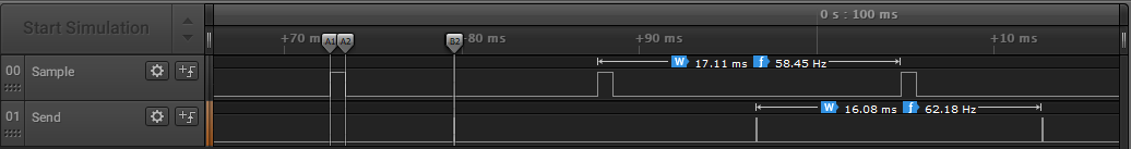
The base station's two tasks, sample and send, were both set to run periodically every 16 milliseconds (approximately 60Hz). As previously mentioned, at the beginning of each task, a digital output pin was set to high, and at the end of each task that same pin was set to low. A Saleae logic analyzer was used to record these pin level changes and measure the durations of the two tasks. From the screenshot below, it can be seen that the time triggered scheduler does not guarantee precise periods. In this instance, the experimental periods of sample and send were 17.11ms and 16.08ms, respectively.

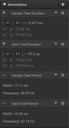
Measurements of the timing markers in the above screenshot are shown below. The execution of the sample task took 907 μs and the execution of the send task took 57.5 μs. It makes sense that sample takes longer because it has to obtain the state of multiple IO devices, as well as apply four low pass filters. In contrast, send simply has to send 9 bytes of data to the built-in UART.

From these measurements, the CPU utilization can be calculated as

Using the measurements below, the CPU is in use 5.66% of the time. That translates to 94% idle time. Note that this is a rough value because of the inconsistency in the scheduler. A more accurate value could be estimated by averaging more samples from the logic analyzer.

Remote Station

The remote station's two tasks, control and receive, were both set to run periodically every 10 milliseconds (approximately 100Hz). As explained above, the higher frequency of the remote station tasks versus the base station tasks ensured an acceptable level of responsiveness in the IO devices and prevented the Bluetooth buffer from filling up.

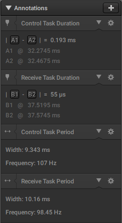
Depicted below, the experimental periods of control and receive were 9.343ms and 10.16ms, respectively.

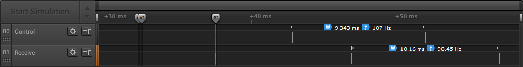
Measurements of the timing markers in the above screenshot are shown below. The execution of the control task took 193 μs and the execution of the receive task took 55 μs. It makes sense that control takes longer because it has to adjust the state of multiple IO devices, whereas receive simply has to read from the UART. It is also worth noting that the computation time of control varies significantly. This is because on some calls the servo is not ready to receive a new position, which decreases the computation cost significantly.

Using the same equation as above, and the measurements listed below, CPU utilization was found to be 2.61%, which translates to roughly 97% idle time.

We also measured our percentage of idle time in software. We used a simple process to determine this.

1. We recorded the time in milliseconds prior to entering the main loop.
2. Each time the time triggered scheduler returns with an idle time duration we add it to an ongoing sum.
3. When we exit the main loop we record the end time in milliseconds.
4. We calculated idle percentage as:

Using this measurement method, we found that on average our base station was idle 93% of the time and our remote station was idle 98% of the time. These correlate closely with the results obtained from the logic analyzer (94% and 97%). Looking at our logical analyzer results it is clear that sampling inputs and controlling the servos is taking up the large majority of the processing time. If we wanted to improve our CPU utilization, this would be our starting point.

Now that we have completed project 1 we are preparing and planning for project 2 where we will expand upon our current TTA, developing it into our own simple real-time operating system.

[1] M. Cheng, "Project 3", Webhome.csc.uvic.ca, 2019. [Online]. Available: https://webhome.csc.uvic.ca/~mcheng/460/spring.2019/p3.html. [Accessed: Apr-2019].

[2] E. Hughes, "Introduction to Fixed Point Math", 2014. [Online]. Available: https://www.youtube.com/watch?v=bbFBgXndmP0. [Accessed: Apr-2019].